Distributed CPU: Zip Fusion Beyond Tensor Parallelism
A research design for treating a cluster of CPU nodes as one pool of compute that re-shapes per graph region: fused one-dimensional lanes that unzip into two-dimensional head-by-context attention at long context, then zip back. The metric is the unresolved span between global synchronization boundaries, priced by a quantitative token-budget and sizing model — and tested by a falsifiable validation ladder, not asserted.
Zip fusion is not implemented in the production runtime. All performance figures on this page are idealized arithmetic, not measurements, and experimental validation is pending. This HTML page is the canonical public design and visual reference; the engineering note
DISTRIBUTED_CPU_ZIP_FUSION.md (in docs/notes/)
is subordinate to it. Nothing here is a supported feature, a measured speedup, or a committed
hardware-compatibility claim.
What it is
- Whole-graph algebraic scheduling: per graph region, pick the representation that maximizes the independent local path before any global synchronization — including work usually treated as implementation detail (quantized unpack, scale decode, local accumulation, SwiGLU, RMSNorm partial statistics, output projection, expert routing, Memory-Tetris residency).
- A cluster as one pool of compute that re-shapes per region: 1-D fused lanes for projections and MLP, a 2-D head-by-context decomposition for long-context attention, and back.
- A measurement program whose deliverable is a topology-versus-context map and a published collective-time fraction — not a single tok/s number.
What it is not
- Not a claim that CKE invented head or context parallelism. Megatron Core, DeepSpeed-Ulysses, Unified Sequence Parallelism, LoongTrain and ATTENTION2D all got there first; the prior-art section below says so plainly.
- Not a promise that link bandwidth equals application throughput. The ~10 µs figure on this page is a division by nominal bandwidth, not a measurement.
- Not implemented. No production code path distributes a model across nodes today; the experimental gates decide whether the idea earns promotion.
The Parallelism Taxonomy: Where Each Method Syncs
Every distributed method shards something different and pays for it at a different synchronization boundary. The honest distinctions that matter for CKE:
- Data parallelism replicates the model and shards requests. It scales throughput across independent requests but never puts two nodes on the same request.
- Tensor parallelism (TP) shards each weight tensor and, in established schedules, pairs column-parallel with row-parallel linears so a layer pays roughly two collectives — not one per operator. All nodes work on the same request simultaneously.
- Pipeline parallelism (PP) shards layers into stages. It is excellent for capacity and for throughput when several microbatches are in flight, but it does not aggregate compute for a single request — one token still flows stage to stage.
- Context / sequence parallelism (CP) shards the token sequence and pays an all-to-all or ring exchange around attention. All nodes work on the same request.
- Expert parallelism (EP) shards MoE experts and synchronizes at routing dispatch and combine per MoE layer.
- Head parallelism shards attention heads and is fully head-independent: each head's softmax is computed locally, heads meet only where the output projection mixes them, and the sole reduction is hidden-state-sized. The online-softmax statistic merge appears only when head parallelism is combined with context parallelism.
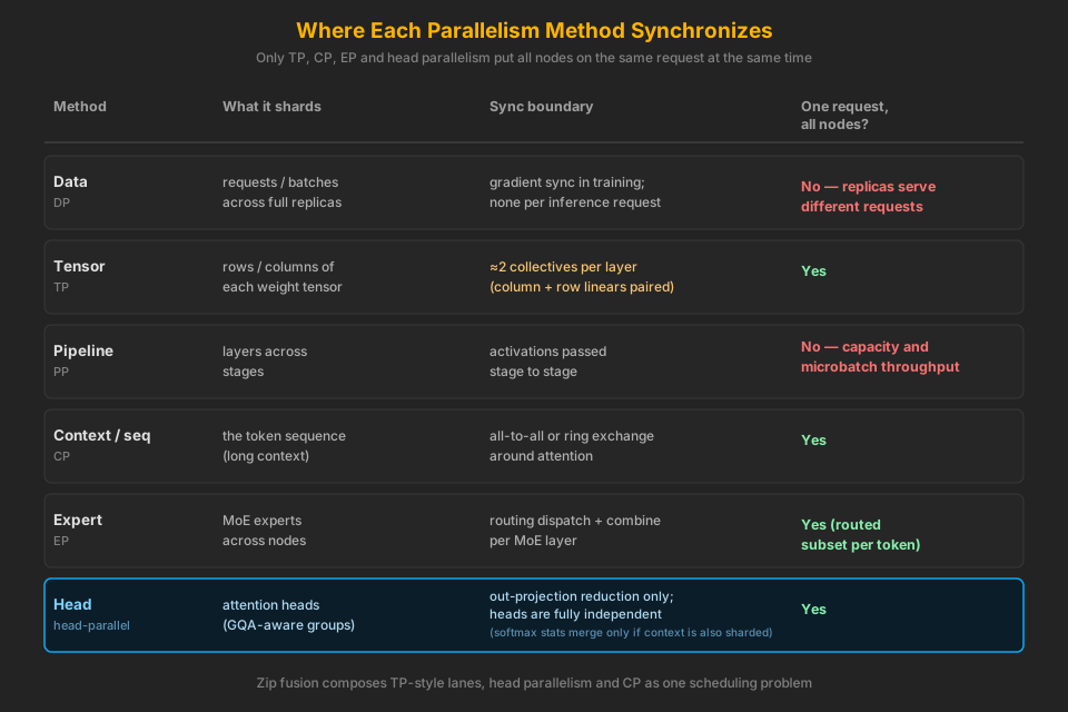
TP, head and context parallelism are the interesting family for latency: they can make every CPU in the cluster work on the same request at the same time. Zip fusion composes them as one scheduling problem instead of three separate flags.
Prior Art, Candidly
CKE did not invent head-shard or context-shard attention, and this page does not claim otherwise:
- Megatron Core combines tensor, pipeline, context and expert parallelism, and treats context parallelism as a first-class way to partition long sequences.
- DeepSpeed provides pipeline, tensor and expert parallelism; its MoE API can distribute experts differently per MoE layer.
- vLLM supports combinations such as data-parallel attention with expert- or tensor-parallel MoE layers.
- DeepSpeed-Ulysses partitions along sequence length and uses all-to-all communication for attention.
- Unified Sequence Parallelism combines Ulysses with Ring Attention.
- LoongTrain explicitly combines head parallelism and context parallelism as a 2-D attention decomposition.
- ATTENTION2D similarly partitions attention along query and key/value dimensions.
The distinctive claim is deliberately narrower: whole-graph algebraic scheduling on CPU-first economics. Rather than exposing named strategies, the scheduler asks, per graph region: what representation lets N CPU nodes execute the longest independent local path before any global synchronization? The unit of distribution is the whole quantized operator subgraph — including packed-weight unpack, scale decode, quantized dot products, local accumulation, SwiGLU, RMSNorm partial statistics, attention-head work, output projection, expert routing and Memory-Tetris residency — not just GEMM or attention. Whether that combination is worth anything is an experimental question, not a marketing one.
What Exactly Is Being Sharded? The Block as a Zipper
Before budgets and topologies, the object itself: a transformer block drawn as a zipper. The hidden state enters replicated on every node (CPU DRAM is plentiful — replication is cheap, communication is not). Each node then runs a vertical local lane — quantized unpack, local QKV GEMM, head-local work (RoPE, QK-norm, attention over its heads), and its own output-projection partial — with zero data movement between lanes. The zipper closes only where the algebra forces it: the output-projection partials must sum into one hidden-state vector. It immediately unzips again for the MLP region and closes once more at the down-projection partials.
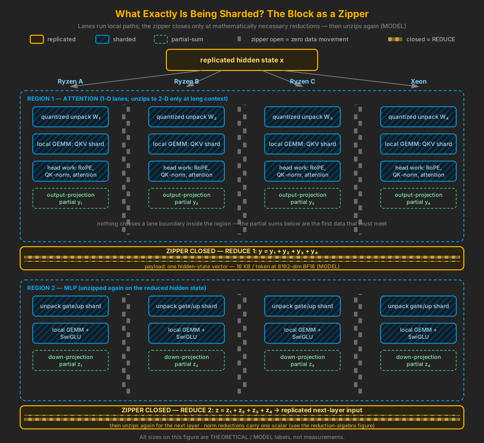
Three tensor states appear, and the scheduler treats them differently: replicated (same bytes on every node — hidden state, norm parameters, routing metadata), sharded (disjoint slices — weight columns, heads, context), and partial-sum (values that are mathematically incomplete until reduced — projection partials, norm statistics). The zip schedule is the discipline of keeping tensors in the sharded state for as long as the algebra allows, and letting the partial-sum state exist only at true dependency boundaries.
The Zip Schedule
The centerpiece. Most of a transformer layer does not need a 2-D decomposition at all: each node can run a fused 1-D lane — unpack its local packed-weight shard, run its QKV shard, its local heads, its local output-projection partial, its local reduction. Crucially, heads are never concatenated into one giant intermediate tensor: each node applies its local output-projection shard to its own attention output, so the first communication boundary is already hidden-state-sized, not attention-sized.
For attention at long context, the decomposition unzips into 2-D — head groups on one axis, context shards on the other — because head count alone eventually stops exposing enough parallelism while the sequence keeps growing. After attention, the schedule zips back to the 1-D lane for the MLP. The cluster is one pool of compute that re-shapes per graph region.
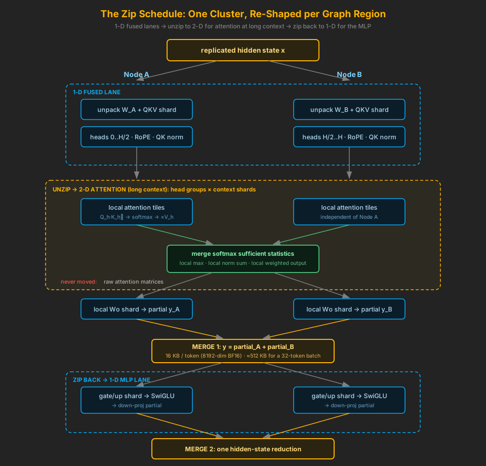
Communication boundaries carry only the mathematically unavoidable reductions:
- Hidden-state-sized partial sums: 16 KB per token at 8192-dimensional BF16 (8192 × 2 bytes); roughly 512 KB for a 32-token batch. Tiny compared with the arithmetic that produced those values.
- Online-softmax sufficient statistics for cross-context attention merges: the local max, the local normalization sum and the local weighted output per partition — never the raw attention matrix.
GQA note. Modern Qwen-like models use grouped-query attention — conceptually 32 query heads against 8 KV heads rather than 32 independent Q/K/V sets. Head sharding must partition query-head groups so the needed KV heads are local or cheaply replicated. Because CPU RAM is plentiful, replicating K/V-head metadata or even some KV data can be preferable to forcing communication — the abundance-of-memory thesis again.
What Must Cross the Fabric: The Reduction Algebra
The synchronization payload is not an implementation choice — it is fixed by the algebra. Split a weight matrix column-wise across \(N\) nodes, \(W = [W_1, W_2, \dots, W_N]\). Each node computes its local product and everything that depends only on it:
\[ Y_i = X\,W_i, \qquad H_i = f(Y_i) \]where \(f\) covers arbitrarily much local work — head-local attention, SwiGLU, quantized unpack and scale decode. No bytes cross the fabric for any of it. Only when the graph needs the output projection does anything meet:
\[ Z = \sum_i H_i\,V_i \qquad \text{REDUCE: one hidden-size vector} \]RMSNorm looks like a global dependency, and it is — but the dependency reduces to a scalar. Each shard accumulates its local sum of squares, and only those scalars ever meet:
\[ s_i = \sum_{j \in shard_i} x_j^2, \qquad s = \sum_i s_i \qquad \text{REDUCE: one scalar} \]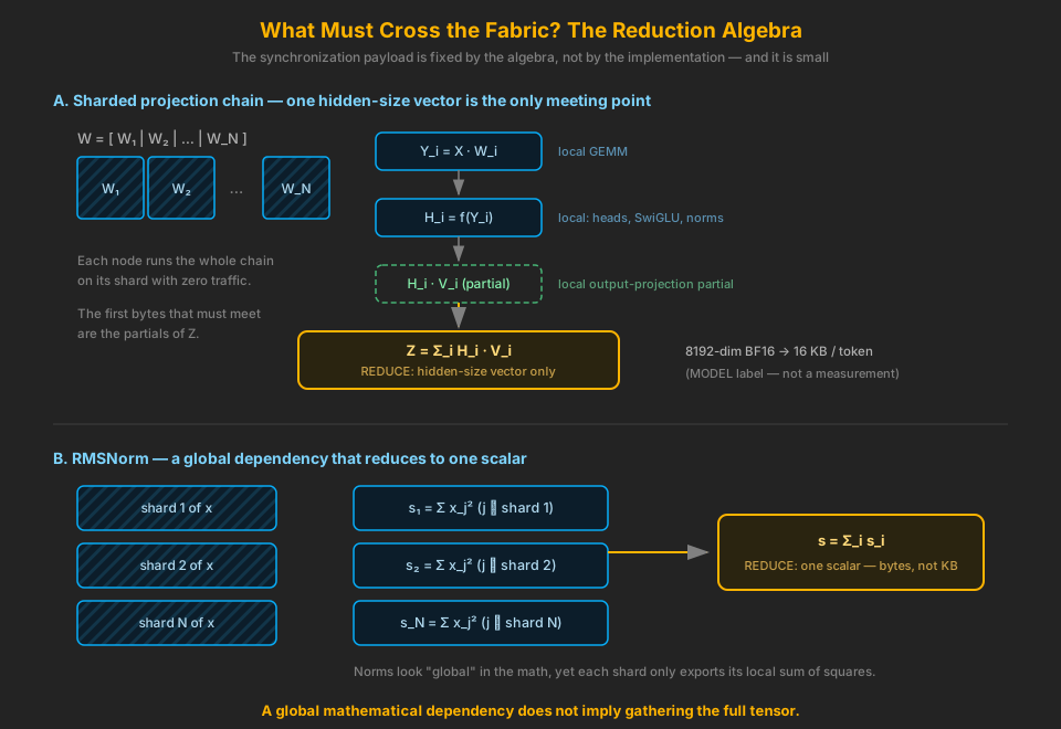
This is the honest foundation of the zip schedule: a global mathematical dependency does not imply gathering the full tensor. The reduction above is also exactly where CKE's zero-tolerance numerical contracts bite — the distributed sum must be specified with the same reduction-order discipline as every other kernel contract, or parity fails. Distribution changes where the tiles run, never the arithmetic.
Two-Dimensional Attention at Long Context
Head parallelism exhausts itself: with 32 heads, 32 nodes means one head per node, and the head axis is spent. At 128K–1M context the sequence is the next parallel axis. A 6-node cluster can decompose as 3 context shards × 2 head groups, each node computing large local attention tiles over 1/3 of the context and 1/2 of the heads, then merging across context partitions with online-softmax sufficient statistics.
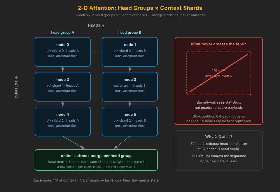
Two honesty constraints at 1M context. First, not every layer needs this: models mix recurrent or local-attention layers (bounded state, no full-context dependency) with global-attention layers, and the mix must be read from the exact model config — never hard-coded into the scheduler. Second, the cross-context merge is exact, not approximate: online softmax rescales each shard's partial statistics before summing, the same algebra a single-node flash-attention kernel uses internally.
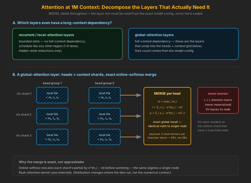
Decode at 1M is not prefill at 1M
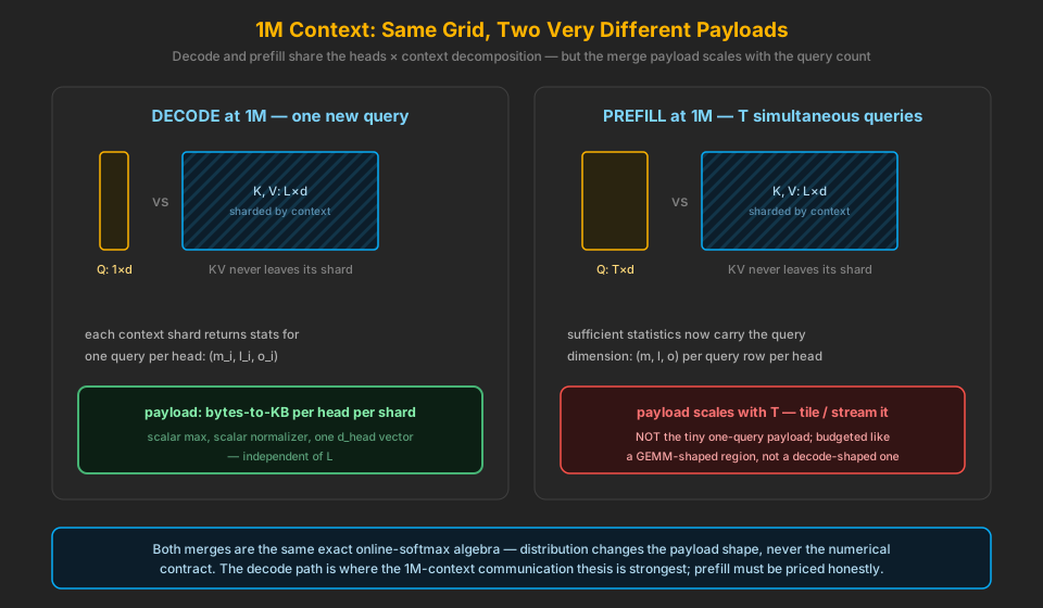
The grid above is shared, but the two phases pay radically different communication over it. At decode there is one new query, \(Q: 1 \times d\), against \(K, V: L \times d\) — each context shard returns the sufficient statistics for that single query per head (a scalar max, a scalar normalizer, one \(d_{\text{head}}\) vector): bytes-to-KB per head per shard, independent of \(L\). This is where the long-context communication thesis is strongest. At prefill, \(T\) queries run simultaneously, so the sufficient statistics themselves carry the query dimension — the merge payload scales with \(T\) and must be tiled or streamed, priced like a GEMM-shaped region rather than a decode-shaped one. Same exact algebra; different payload shape. Any 1M-context claim on this page that does not name its phase is incomplete.
The Metric: Synchronization Boundaries per Layer
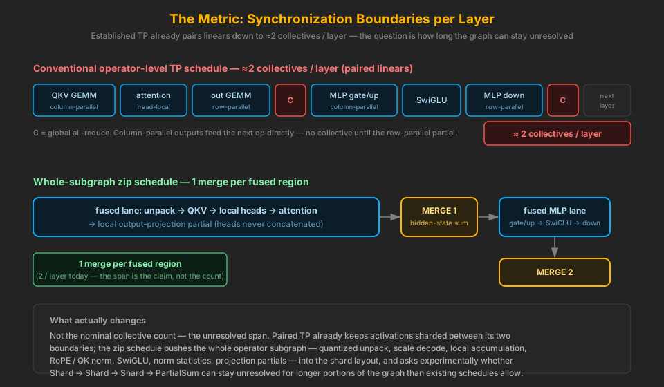
“We support TP=2” says nothing about how often nodes stop to agree. The useful metric is
global synchronization boundaries per layer — and the honest baseline is
stronger than a strawman: established TP schedules already pair column-parallel with row-parallel
linears, so a conventional layer pays roughly two collectives, not one per
operator. The real contrast is not the nominal count but the unresolved span:
paired TP keeps activations sharded between its two boundaries, while the zip schedule pushes the
whole operator subgraph — quantized unpack, scale decode, local accumulation, RoPE / QK norm,
SwiGLU, norm statistics, projection partials — into the shard layout. The experimental
question is whether Shard → Shard → Shard → PartialSum can stay
unresolved for longer portions of the graph than existing schedules allow.
The Token Budget: A 20 ms Worked Example (MODEL)
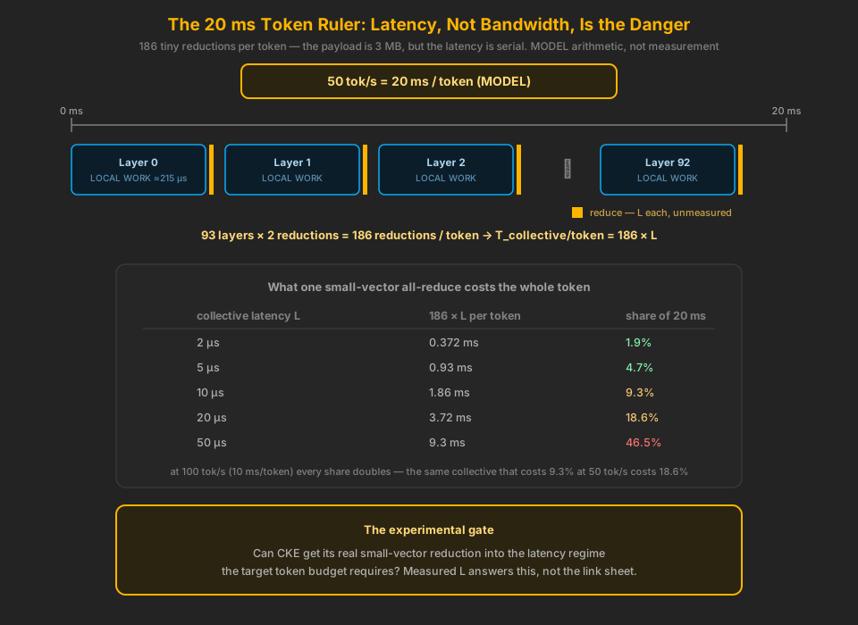
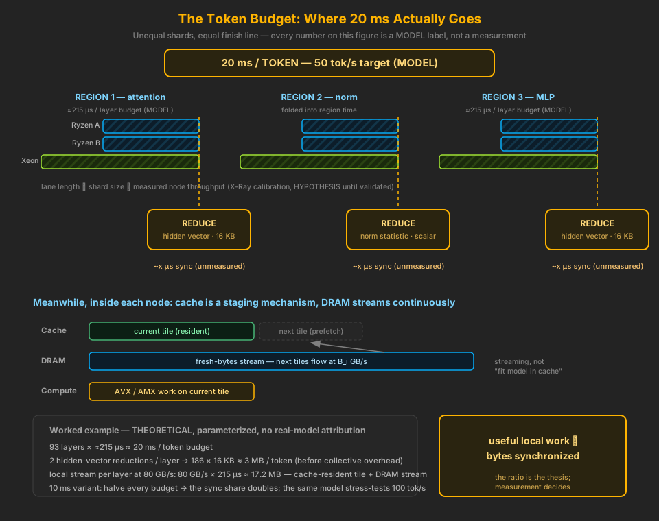
The figures so far say what moves; this section prices it. Take a 50 tok/s decode target — 20 ms per token — and a parameterized example model: 93 layers, hidden dimension 8192 in BF16. These are THEORETICAL model labels with no real-model attribution; the point is to show the arithmetic a planner would run, not to benchmark anything.
The per-layer budget is a division:
\[ \frac{20\ \text{ms}}{93\ \text{layers}} \approx 215\ \mu\text{s / layer} \]Against that budget, the synchronization payload is tiny. A hidden-state reduction at 8192 dimensions in BF16 is 16 KB; at two such reductions per layer (attention out-projection, MLP down-projection) the whole token pays:
\[ 93 \times 2 \times 16\ \text{KB} \approx 3\ \text{MB / token} \quad \text{(before collective-algorithm overhead)} \]Meanwhile each node must stream its weight shard from DRAM inside the same 215 µs. The first-class variable is fresh bytes — the bytes DRAM must actually deliver, after cache reuse:
\[ B_{\text{fresh}} = B_{\text{required}} - B_{\text{cache hits / reuse}} \]This is why a large-cache node can outperform what its nominal two-channel DRAM bandwidth suggests on some regions: the planner cares about \(B_{\text{fresh}}\), not total weight bytes. At a sustained stream bandwidth \(B_i\), the fresh bytes a node can absorb per layer are:
\[ B_{\text{fresh}}\ \text{/ layer} = B_i \times 215\ \mu\text{s} \qquad \text{e.g. } 80\ \text{GB/s} \times 215\ \mu\text{s} \approx 17.2\ \text{MB} \]That is the sense in which cache is a staging mechanism, not a model residence: the current tile is cache-resident while DRAM streams the next one, and AVX/AMX compute consumes the current one — compute current tile in parallel with fetch next tile. A 100 tok/s variant simply halves every budget — which doubles the sync share of wall time, making the same model a stress test of the communication path.
The latency arithmetic: why 3 MB is not the story
The 3 MB/token payload sounds trivially cheap — and on bandwidth it is. The danger is latency, paid serially. The reductions do not overlap each other; each layer's boundary waits for its collective, so per-token synchronization cost is:
\[ T_{\text{collective / token}} = 186 \times L_{\text{collective}} \]At \(L = 10\,\mu s\) that is 1.86 ms — 9.3% of the 20 ms budget gone to waiting, before any collective-algorithm overhead. At a 100 tok/s target the same 10 µs collective costs 18.6%. The whole distributed-CPU thesis therefore reduces to one measurable question: can CKE get its real small-vector reduction into the latency regime the target token budget requires? The ruler below makes the budget, the serial ticks and the latency table one picture.
Decode vs Prefill: Same Weights, Different Bottlenecks
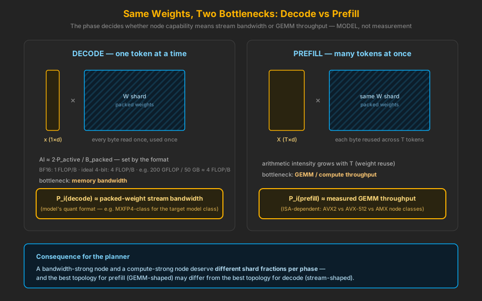
One model, two operating points. Decode multiplies a one-token vector by the weight matrix: every packed weight byte is read once and used once, and the region is bandwidth dominated. The arithmetic intensity is set by the format, not a universal constant — the honest expression is:
\[ AI_{\text{decode}} \approx \frac{2 \times P_{\text{active}}}{B_{\text{packed weights}}} \]FP32 gives 0.5 FLOP/byte, BF16 gives 1, and ideal packed 4-bit weights give \(\approx 4\) FLOP/byte before scale/block metadata, unpack overhead and activation traffic — e.g. a 100B-parameter model at \(\approx\)50 GB packed streams 200 GFLOP against 50 GB, \(\approx 4\) FLOP/byte. CKE computes this from the actual format rather than assuming one. Prefill multiplies a token matrix by the same weights: each byte is reused across \(T\) tokens, arithmetic intensity grows with \(T\), and the region is GEMM/compute dominated. Node capability is therefore phase-dependent:
\[ P_i^{\text{decode}} \approx \text{packed-weight stream bandwidth}, \qquad P_i^{\text{prefill}} \approx \text{measured GEMM throughput} \]“Packed-weight stream bandwidth” means whatever quant format the target model ships in (an MXFP4-class format for the model class this research targets) — it is a property of the model artifact and the node's memory system, not a CKE capability claim. The planner consequence: a bandwidth-strong node and a compute-strong node deserve different shard fractions per phase, and the best prefill topology may differ from the best decode topology on the same hardware.
Prefill First, Then One Matrix-Work Scheduler
Prefill is the cleanest place to prove CKE's deterministic scaling story first. A prefill region multiplies a token matrix by the weight matrix, \(X_{B \times d}\,W_{d \times k}\), so the same weight tile is reused across \(B\) token rows and arithmetic intensity rises with \(B\). When the region is genuinely dense — compute time exceeds streaming time:
\[ \frac{F_r}{P} > \frac{B_{\text{fresh},r}}{BW} \quad\Longrightarrow\quad T_r \approx \frac{F_r}{P_{\text{cluster}}} + T_{\text{sync}} \]— the first objective becomes simple to state: maximize sustained useful GEMM throughput across the cluster, and check whether adding a node adds its measured compute minus a small, visible synchronization term. No bandwidth cliff, no cache phenomenology — those enter later, on their own measured terms.
Decode then stops being a separate architecture. Batch-1 decode multiplies one token row by the weights, but continuous batching packs every runnable sequence into the same product:
\[ X = \begin{bmatrix} x_1 \\ x_2 \\ \vdots \\ x_B \end{bmatrix}, \qquad XW \]As \(B\) grows, the workload slides along a continuum — GEMV-like, small GEMM, large GEMM — and CKE needs one matrix-work scheduler, not a “prefill runtime” and a “decode runtime”. The scheduler's question is always the same: how many compatible activation rows are ready for this weight region, and which tiling and sharding gives the shortest critical path — continuously packing available token work toward dense GEMM while respecting per-user latency constraints.
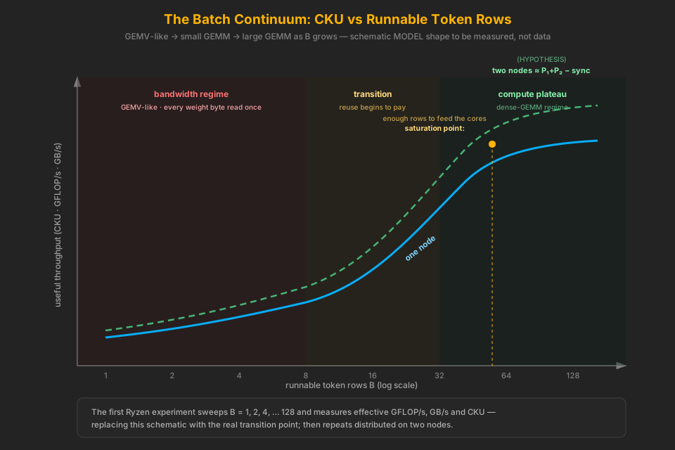
The transition point on that curve is an experimental deliverable, not an assumption: MXFP4-class unpacking, scaling, tile shapes, ISA utilization and cache behavior decide where a real node stops being bandwidth-bound. The first Ryzen experiment sweeps \(B = 1, 2, 4, \ldots, 128\) and measures effective GFLOP/s, effective GB/s and CKU per point; the two-node repeat should show the plateau move to approximately \(P_1 + P_2\) minus synchronization if the scheduler is honest.
KV and recurrent state stay special — but as regions, not as an architecture. Even when batching makes the dense projections GEMM-like, every sequence carries independent state, \(KV_1, KV_2, \ldots, KV_B\), so attention has a different data-access structure from the projections. CKE treats it as another region in the same schedule — dense projection, local attention/KV work, small reduction if required — and lets X-Ray report which regions ran below peak and why. Models with recurrent or linear-attention layers may shrink the long-context KV burden; that is a per-model measurement, never a CKE core assumption. The overall objective stays singular: keep as much of the execution graph in the dense-GEMM regime as possible, and optimize the whole architecture around that rather than around the worst batch-1 decode case.
Communication Must Be Measured
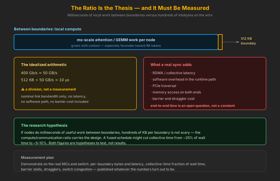
The fast-switch intuition, stated honestly: 512 KB at a nominal 400 Gb/s (≈ 50 GB/s) link serializes in about 10 µs — and that figure is a division, not a measurement. Real end-to-end synchronization adds RDMA/collective latency, software overhead, PCIe traversal, memory access and barrier cost. None of that is in the division.
The thesis stands on the ratio, not the absolute number: if each node performs milliseconds of useful attention/GEMM work between boundaries, hundreds of kilobytes of communication is not scary — and at 1M context the compute/communication ratio can become particularly favorable. But this is a research hypothesis. It must be demonstrated on the real NICs and switch, not assumed from a link sheet, and the measurement plan below publishes the collective-time fraction whatever it turns out to be.
The synchronization root is also a constraint
One appealing small-cluster shape is a star: Ryzen leaf nodes with direct high-speed links to a PCIe-rich Xeon hub, which hosts the reduction. The appeal is determinism — CKE knows exactly which link each rank uses, its measured latency and bandwidth, where the reduction happens and how long broadcast takes, with no external switch fabric whose congestion must be modeled. And the hub is asked to combine partial results, not model tensors: leaves keep weights local (\(B_{\text{local weights}} \gg B_{\text{sync}}\)), send their partials, and the hub computes \(z = \sum_i z_i\) and broadcasts \(z\).
But the star just moves the constraint — it never deletes it. The hub's PCIe bandwidth, NIC DMA capability, memory system, reduction compute and per-message processing bound \(T_{\text{star}}(N)\); what is perfectly reasonable at 4 leaves may fail at 32. The planner must therefore treat topology itself as a variable — star, hierarchical tree of hubs, or peer-to-peer reduction — and say, at a measured node count, “the hub is now the active constraint; change topology.” This is the constraint model applied to the fabric: every topology has a slowest active boundary, including the one CKE just created on purpose.
Streaming reductions: keep the pipeline moving
Reductions are associative, so the hub need not wait for every partial before doing anything: reduce-as-arrive (\(z^{(1)} = z_1 + z_2\), then \(z^{(2)} = z^{(1)} + z_3\), …) overlaps network reception with reduction compute, and sufficiently segmented results can begin broadcast as soon as portions resolve. “Receive everything → reduce everything → send everything” becomes a streaming reduction — the flowing-pipeline discipline of the constraint model applied to the collective itself. One hard boundary remains: reduction order is part of the numerical contract, so any streaming order must be fixed, declared and certified — never an opportunistic arrival-order sum.
CPU-First Economics: Spend DRAM to Eliminate Communication
GPU frameworks shard because HBM is scarce — state often cannot be replicated. CPU nodes can carry 150 GB, 256 GB, 512 GB or eventually terabytes of DRAM, which inverts the optimization objective: CKE can deliberately spend memory to eliminate communication:
- replicate the hidden input, norm parameters and routing metadata;
- keep multiple packed layouts of the same weights;
- replicate GQA KV heads for locality instead of communicating them;
- cache hot experts on several nodes.
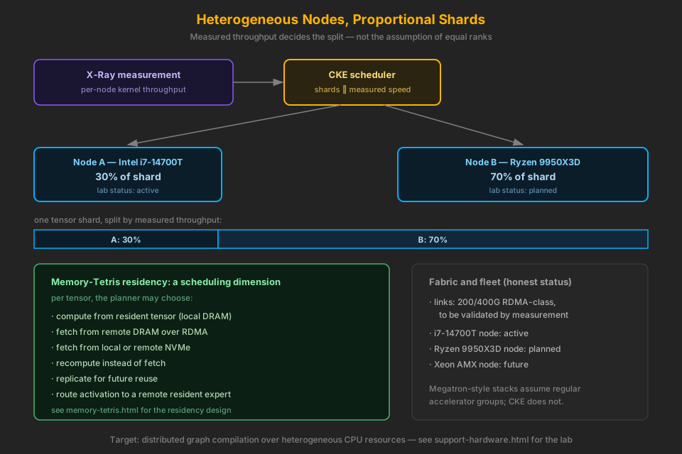
Memory Tetris adds the dimension the mainstream parallelism literature usually does not center: tensor residency itself is part of scheduling. Per tensor, the planner could choose to compute from a resident tensor, fetch from remote DRAM over RDMA, fetch from local or remote NVMe, recompute, replicate for future reuse, or route the activation to a remote resident expert. See Memory Tetris: DRAM as a Tensor Cache over NVMe for the residency design — itself a research design at the same status as this page.
Heterogeneous Topology
Megatron-style systems generally assume fairly regular accelerator groups. The CKE lab fleet is explicitly heterogeneous — an Intel i7-14700T node (active), a Ryzen 9950X3D node (planned) and Xeon AMX hardware (future) — so equal ranks are the wrong default. Shards should be proportional to X-Ray-measured throughput: Node A might take 30% of a tensor shard and Node B 70%, because X-Ray measured them that way. The target is distributed graph compilation over heterogeneous CPU resources. See Support Hardware for the lab fleet.
The sizing model (OPTIMISTIC LOWER BOUND)
Heterogeneous sharding needs a quantitative rule, not a vibe. Let \(P_i\) be node \(i\)'s
X-Ray-measured CKE throughput for the relevant region — and note that
\(P_i\) is really \(P_i(r, \text{phase}, \text{dtype})\): stream bandwidth for decode-shaped
regions, GEMM throughput for prefill-shaped regions, something like
\(f(BW_{\text{KV}}, F_{\text{attention}})\) for long-context attention — never nominal
FLOPS, and not one constant per node. The same Xeon/Ryzen ratio does not apply everywhere,
which is exactly where this differs from a static --tensor-split 0.2,0.2,0.6:
the shard size is operator- and phase-dependent. The fractions follow directly:
Region time is bounded below by whichever resource saturates first — on fresh bytes, not total weight bytes — plus the synchronization the algebra forces, which is a measured, node-count-dependent term \(C_r(N)\):
\[ T_r = \max\!\left( \frac{B_{\text{fresh},r}}{\sum_i BW_{i,r}},\ \frac{F_r}{\sum_i F_{i,r}} \right) + C_r(N) \]Elevated to the headline equation — the whole distributed-CPU hypothesis in one line:
\[ \boxed{\; T_{\text{token}} = \sum_r \left[ \max\!\left( \frac{B_{\text{fresh},r}}{\sum_i BW_{i,r}},\ \frac{F_r}{\sum_i F_{i,r}} \right) + C_r(N) \right] \;} \] \[ \text{tok/s} = \frac{1000}{T_{\text{token}}\ \text{(ms)}} \]where \(B_{\text{fresh},r}\) and \(F_r\) are the region's fresh bytes and FLOPs. Two labels apply to every use of these equations on this page: OPTIMISTIC LOWER BOUND — measured time will be ≥ predicted, because the max() ignores overlap penalties, stragglers, collective algorithms and software overhead; and THEORETICAL — the model exists to be validated or falsified by the ladder below, not to advertise a number.
On heterogeneous nodes the region finishes at the slowest lane's time, not the fastest: lanes measuring 180, 182, 179 and 95 µs produce a ≈182 µs region, with the fast node wasting 87 µs at the barrier. Shard assignment is therefore the critical-path minimization:
\[ \underset{s_1,\dots,s_N}{\arg\min}\ \left[ \max_i T_i(s_i)\ +\ T_{\text{sync}}(N, B) \right] \quad \text{subject to } \sum_i s_i = 1 \]Rebalance until the lanes tie — 180, 181, 179, 180 — and \(\max_i T_i\) is minimized. This equation is the distributed instance of the CKE Constraint Model, which defines the shared per-resource clocks and the exposed-versus-hidden vocabulary this page uses throughout.
The Topology-versus-Context Thesis
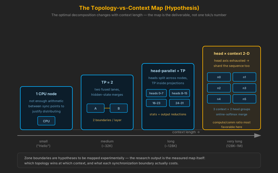
For a tiny decode prompt there is not enough arithmetic between synchronization points to justify distributing aggressively. As context grows — 32K, 128K, 500K, 1M — the attention work becomes enormous and the optimal topology plausibly changes: one node for small context, TP=2 for medium, head-parallel plus TP for long, and head-by-context 2-D for very long. The interesting output of this research is the measured map of which topology wins at which context — not a single tok/s figure.
Experimental Plan and Promotion Gates
Same rigor as Memory Tetris: ordered experiments, each with a promotion gate, every result cell not yet certified until measured and recorded to CKE's evidence standard.
| Experiment | What it measures | Result | Status |
|---|---|---|---|
| Single-node baseline | fully resident model; per-region kernel times | — | Not yet certified |
| Two-node TP reference | conventional TP=2; percentage of wall time in collectives | — | Not yet certified |
| Hyper-fused schedule | boundaries per layer; total sync time; collective-time fraction | — | Not yet certified |
| Head × context 2-D | 6-node 3×2 grid with online-softmax merging at long context | — | Not yet certified |
| Token-row sweep | B = 1…128 batch continuum; effective GFLOP/s, GB/s and CKU per point; locates the bandwidth-to-compute transition; repeated on two nodes | — | Not yet certified |
| Numerical parity | distributed schedule vs single-node baseline under the zero-tolerance numerical contract rules; layer/checkpoint outputs, not just tokens | — | Not yet certified |
| Topology-vs-context map | winning topology per context length, published as a map | — | Not yet certified |
The hypothesis to test — not a result
If two nodes running a conventional TP implementation spend, say, ~25% of wall time in collectives, a hyper-fused schedule might cut that to ~5–10%. Both numbers are hypotheses the experiments are designed to confirm or refute, and the collective-time fraction gets published either way.
The validation ladder: prediction first, measurement second
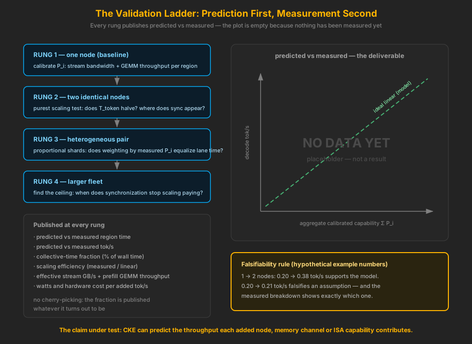
The experiments above order the work; the ladder orders the fleet. Each rung adds compute the sizing model claims it can price, and each rung publishes the same evidence pack: predicted vs measured region time, predicted vs measured tok/s, collective-time fraction, scaling efficiency, effective stream bandwidth and prefill GEMM throughput, watts, and hardware cost per added tok/s. The fraction is published whatever it turns out to be — no cherry-picking.
The headline question — sharper than “CPU vs GPU”
Can transformer latency scale approximately with aggregate calibrated CPU capability until synchronization becomes the ceiling?
This is deliberately falsifiable. If one node decodes at 0.20 tok/s (hypothetical example number) and two deliver 0.38, the sizing model is supported. If two deliver 0.21, an assumption is falsified — and the per-region breakdown shows exactly which one: the bandwidth term, the GEMM term, or the sync term. Either outcome is a publishable result, because the research claim is not “CPU is faster than GPU” but CKE can predict how much useful transformer throughput each added node, memory channel, cache hierarchy or ISA capability contributes to the compute fabric.
Failure modes to measure
- Barrier stalls — every boundary is a place where one slow node holds the cluster.
- Stragglers on heterogeneous nodes — does proportional sharding actually equalize lane time?
- GQA KV replication cost — when does replicating KV beat communicating it?
- Switch congestion — does the fabric stay cheap at 6+ nodes, or become the boundary condition?
Related Pages
- The CKE Constraint Model — the umbrella math: per-resource clocks, exposed-vs-hidden transfers, and the critical-path scheduler this page instantiates
- Memory Tetris — the residency design that makes tensor placement a scheduling dimension
- Support Hardware — the heterogeneous lab fleet this research targets
- v8 Numerical Contracts — the zero-tolerance parity rules every distributed schedule must satisfy
- Kernel Maps and Provider Selection — how physical kernels are selected today, per node
- Scaling Philosophy — the CPU-only, Linux-first hardware bet behind this research
- Research Tracker — other proposed techniques and their status