The CKE Constraint Model

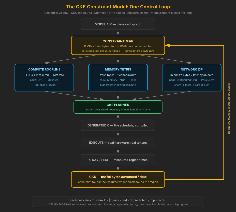
Theory of Constraints expressed as runtime math. Every generated region has several clocks running — compute, cache, DRAM, network, storage — and the region takes as long as the slowest required path plus the synchronization that could not be hidden. Scaling says why, CKU measures, Memory Tetris places, Distributed Zip parallelizes — and measurement closes the loop.

One Theory, Four Pages

Four CKE documents have been circling the same idea from different altitudes. They are one theory:

The Per-Region Clocks

For any generated region \(r\), a CPU node has several clocks running concurrently. Compute:

DRAM, on fresh bytes (what DRAM must actually deliver after cache reuse):

Network, where latency usually dominates the payload:

and, when Memory Tetris tiering is involved, storage:

When independent clocks overlap, region time is approximately their maximum, not their sum — plus whatever synchronization could not be hidden:

The slowest required path is the constraint. Optimizing any other clock buys nothing until the constraint moves — that is Goldratt's observation, restated as runtime math.

Exposed vs Hidden: The Overlap Equation

A transfer only costs wall time when it is exposed — longer than the work that could have hidden it. One equation covers every tier:

Instantiated per path:

A 250 µs NVMe prefetch under 300 µs of compute contributes zero exposed storage time; a 500 µs transfer under the same compute exposes 200 µs. Memory Tetris's residency choices, the zip schedule's independent lanes, and ordinary cache prefetch are all the same move: grow the overlap window or shrink the transfer until the exposure is zero.

Shape the Clocks: The Flowing Pipeline

The maximum in the core equation is a bound, not the goal. The goal is to shape the work assigned to every node so the clocks line up — during a region, \(T_{\text{compute},i} \approx T_{\text{stream},i} \approx T_{\text{prefetch},i}\), with synchronization from neighboring regions hidden or extremely short. The contrast is between a stall pipeline (fetch → stall → compute → stall → sync) and a flowing one, where DRAM streams continuously, the cache prefetches \(N+1\) and \(N+2\) ahead of use, the CPU never waits, and the sync rides the boundary:

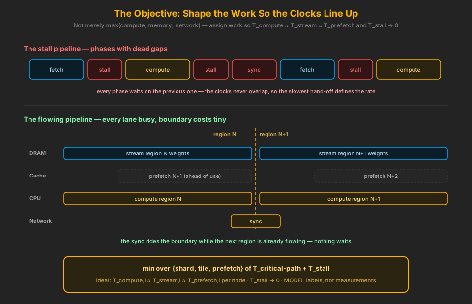
The optimization target is therefore not a single roof but a schedule:

Supply meets demand: the node gets what it can finish on time

A node does not get “its fair share” — one fourth because there are four nodes. It gets what it can finish before the boundary. If a Ryzen sustains \(BW_i = 80\) GB/s on the actual CKE packed-weight path and its kernel can process a tile in 150 µs, the memory system can only supply \(80 \times 150\,\mu s = 12\) MB of fresh bytes in that window. With 4 MB of useful hot data already in cache, the region can operate on roughly 16 MB. Assign 30 MB and the CPU waits on memory; assign 5 MB and memory capacity sits unused while the CPU starves. The planner searches for:

— arithmetic demand matched to the memory supply rate (all figures MODEL labels).

Cache as a queue: elasticity between unequal rates

When arithmetic is the slower clock — \(T_{\text{fetch}} = 100\,\mu s\) against \(T_{\text{compute}} = 250\,\mu s\) — memory gets ahead, and a large cache earns its keep in a second way: it is a queue between two unequal rates, DRAM producer → LLC buffer → CPU consumer. While the CPU computes tile \(N\), DRAM can prefetch \(N+1\) and possibly \(N+2\), capacity and associativity permitting. When the CPU is faster than DRAM, the planner's moves are the Theory-of-Constraints levers: smaller tiles, more reuse, another memory-producing node or channel, or a restructured operator.

The Refined Core Equation

With the overlap vocabulary in hand, the core equation sharpens from a max-of-roofs to a critical path plus exposed stall:

and CKE's two jobs follow directly: minimize \(T_{\text{exposed-stall}}\) (hide everything hidable) and minimize \(\max_i T_i\) (balance what cannot be hidden). Theory of Constraints plus scheduling, in one line each.

The Heterogeneous Scheduler: Minimize the Critical-Path Maximum

On heterogeneous nodes the region does not finish at the fastest lane's time — it finishes at the slowest lane's time, plus synchronization. If the lanes measure 180, 182, 179 and 95 µs, the region takes ≈182 µs \(+\ T_{\text{sync}}\), and the fast node wastes 87 µs waiting. The planner's objective is therefore the critical-path maximum:

where \(s_i\) is node \(i\)'s shard fraction and \(T_i\) follows from its measured \(P_i(r, \text{phase}, \text{dtype})\). Rebalance until the lanes tie — 180, 181, 179, 180 — and \(\max_i T_i\) is minimized. This is the deterministic form of the distributed-CPU sizing model: shard geometry derived from measured capability, not static ratios.

Balanced completion time, not balanced bytes

The per-node estimate credits cache-resident reuse \(C_i\) against the fresh-byte term:

and the planner solves \(T_1 \approx T_2 \approx \dots \approx T_N\) subject to \(\sum_i s_i = 1\). Note what this does not do: it does not split bytes by bandwidth ratio. With stream rates 80 : 80 : 400 GB/s but compute rates 2 : 2 : 8 TF/s, the correct split is 80 : 80 : 400 only if the region is bandwidth-bound — for a compute-bound region the 2 : 2 : 8 ratio governs, and for anything in between the max() decides per node. The goal is balanced completion time; the byte split is a consequence, not the objective.

Worked Example: One Ryzen Region (MODEL)

A parameterized example, all labels THEORETICAL. DDR5-5600 dual channel:

A ConnectX-class fabric at a nominal 400 Gb/s:

The hierarchy reads cache \(\gg\) 89.6 GB/s DRAM \(>\) 50 GB/s network — but the network does not limit the transformer to 50 GB/s, because it does not carry the same bytes as DRAM. That is the central zip insight. Suppose a 200 µs region consumes 18 MB of local weight data and synchronizes only 16 KB at its boundary:

Network bandwidth is nearly irrelevant; the network latency is not. With a collective latency of 8 µs (unmeasured, MODEL):

This is the kind of calculation CKE should generate for every region — then replace with a measurement. Note how it connects to the token ruler: 186 such boundaries per token make the \(L_{\text{collective}}\) term, not the 0.32 µs of transmission, the term to engineer down.

CKU Refined: The Critical-Path Unit

The CKU roofline already bounds a node by the minimum of its memory, compute and network roofs. The zip schedule refines what “network roof” means: not all active bytes cross all roofs. A node may process \(B_{\text{local}} = 18\) MB while synchronizing only \(B_{\text{sync}} = 16\) KB. The byte classes have different paths, so CKU becomes a per-path vector:

and effective throughput is constrained by the critical path, not by pretending every byte crosses every roof:

CKU is then the observable result of the scheduler — the number the control loop tries to raise by moving the constraint.

“Deterministic” Means Predictable

CKE knows the exact graph, exact tensor shapes, exact lifetimes, exact planned placements, exact communication boundaries and calibrated machine capabilities. It can therefore produce an execution schedule and predict its critical path:

Prediction error becomes a first-class metric:

The research program in one sentence: keep shrinking \(E\). If CKE predicts 2.4 tok/s and measures 2.2, the system model is good; add a node, change the shard geometry, predict 4.1, measure 3.9 — each cycle is a validated or falsified claim about the constraint map (illustrative numbers, not results). That is deterministic computing in a stronger sense than deterministic kernels: the runtime knows what it is about to cost.

The Control Loop

The Planner Discipline

Each resource — arithmetic, cache, DRAM, NUMA, network, storage, synchronization — presents the same quotient:

and the planner attacks the active constraint in a fixed order:

1. Reduce required work — smaller payloads, fewer boundaries, dead-tensor elimination.
2. Overlap independent work — grow the window that hides the transfer.
3. Rebalance shards — minimize the critical-path maximum across heterogeneous nodes.
4. Eliminate unnecessary movement — residency, replication and placement choices.
5. Minimize exposed synchronization — latency on the boundary, not bandwidth, is the term to engineer down.
6. Add hardware only then — when the remaining constraint is physical, and the model says which one.

Related Pages

• Scaling Philosophy — why the constraint, not the peak, is the unit of progress
• CKE Throughput Unit — the measurement the loop optimizes
• Memory Tetris — placement: hiding slower tiers behind useful work
• Distributed CPU: Zip Fusion — parallelization: the sizing model, token budget and validation ladder
• v8 Numerical Contracts — the parity rules every schedule must satisfy
• Research Tracker — status of all proposed techniques